Worksheet for Computing K-Apollonian and Schmidt Arrangement pictures

Summer 2017, Version 1.0

Coding: Katherine E. Stange

Algorithms: Katherine E. Stange and Daniel Martin

Licensed under Attribution-NonCommercial-ShareAlike 4.0 International

The embedded Sage code runs on the Single Cell Sage Server, which has limitations -- some images won't display (try clicking broken image icon), or get cut off. Some computations take a minute or two or may time-out on the single-cell server. Load it into your own version of Sage to play around with more flexibility.

Download the Sage Worksheet if you desire.

To run the code on this webpage, first evaluate the following cell, which loads all the routines. Then play with the various other cells to create pictures.

Instructions for Using The Code:

Usage:

Step 1) Precompute circles.  The entry "dis" is the square root determining the field (-1 = Gaussian, -3 = Eisenstein etc.).  The other entries bound the curvature and the absolute value of the centre coordinates.  This is a time-intensive step for detailed pictures, so save the resulting list for future use.  So do this once and then do Steps 2-5 as desired using the result.

precompute_circles( dis, curvature_bound, xmax, ymax )

Step 2) Filter circles.  You can either specify a rectangle (using xmin,xmax,ymin,ymax) or a circle by specifying center and radius.  The rectangle or circle is used as the region in which circle centres are allowed.  You must feed in the output of Step 1 (here as "coords"), as well as "dis" as in Step 1.  This will filter the circles produced in Step 1 according to your desires.  It won't compute new circles, so curvature_bound should be less than or equal to what you specified in Step 1, for example.

filter_circles_rectangular( dis, coords, curvature_lower_bound, curvature_upper_bound, xmin, xmax, ymin, ymax, filter_down=False )

filter_circles_circular( dis, coords, curvature_lower_bound, curvature_upper_bound, xctr, yctr, radius_squared, filter_down=False )

Step 3) Create picture object. 

• You can use either "disk" or "circle" or "combo" by specifying object_type. 
  
• If using circles, you can use circle_colour_scheme and its associated parameter list, as well as a circle_transparency_scheme and its associated parameter list.
• If using disks, you can use disk_colour_scheme and its associated parameter list, as well as a disk_transparency_scheme and its associated parameter list.
  
• The parameter list for modular_colour scheme is of the form [ palette, [modulus, multiplier, translation] ]. 
  
• If using prime_colour, specify just [ palette ] (which should have at least two colours) for the parameter list. 
  
• For transparency, you have the option of constant_transparency (then parameters are [alpha] 0=transparent, 1=solid), or increasing_transparency or decreasing_transparency.  In the increasing/decreasing case, the parameters are [ upper_bound_on_alpha, translation ] (see the code above for the formula). 
  
• If you choose gradient_disk for the disk_colour_scheme, then disk_transparency_schemes are ignored.  The gradient_disk needs a parameter list like [colour_scheme1, colour_parms1, colour_scheme2, colour_params2, fact], where fact is a factor controlling how fine the gradient is.  Higher fact means smoother gradient.
• sort_up can be set to False in order to pile larger disks on smaller disks
• circle_thickness can be controlled
• line_range is set to a positive number to give more lines (otherwise lines -- curvature 0 -- are not shown).  Increase until all the lines needed are appearing. If this is used, dis should be set to the discriminant in order to compute lines correctly.
  

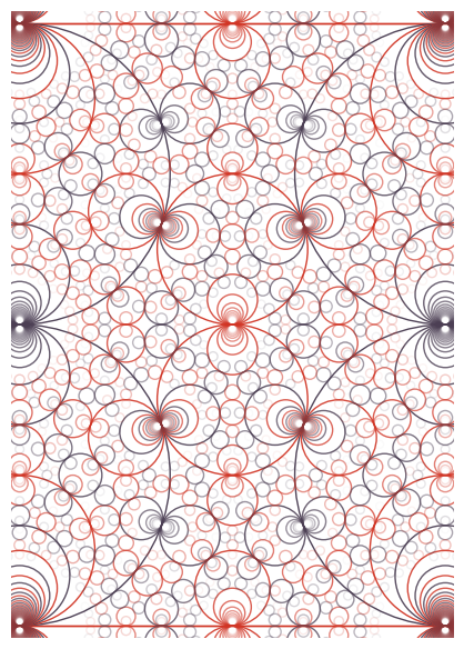
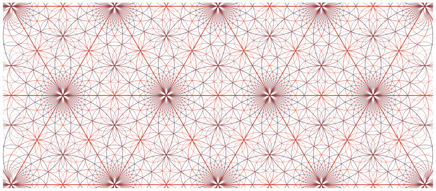
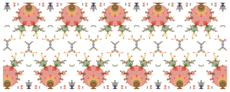
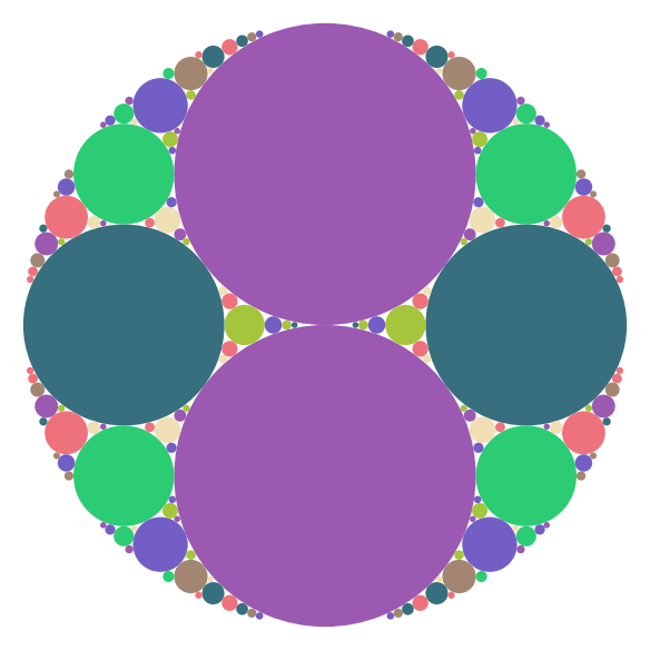
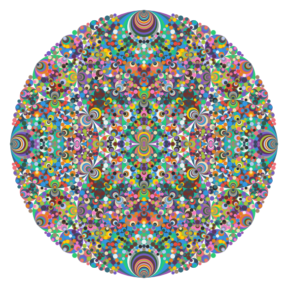
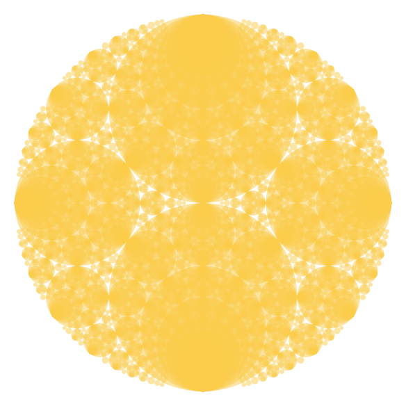
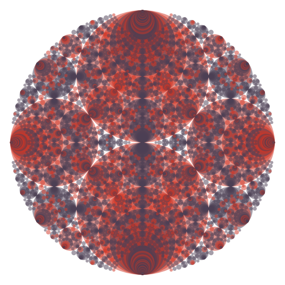
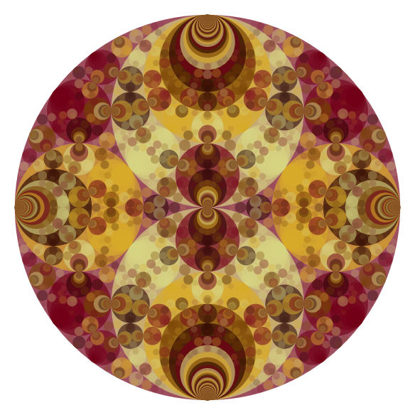
circle_picture( circle_list, object_type="circle", circle_colour_scheme=modular_colour, circle_colour_parameter_list=[colour_cu,[2,0,1]], circle_transparency_scheme=constant_transparency, circle_transparency_parameter_list=[1], disk_colour_scheme=modular_colour, disk_colour_parameter_list=[colour_cu,[1,0,0]], disk_transparency_scheme=constant_transparency, disk_transparency_parameter_list=[1/2], circle_thickness=1, sort_up=True, line_range=0, dis=-1)

Step 4) Display the object.  You can add things like "axes=False" to beautify the output.

pic.show(axes=False)

Step 5) Save your image.  It will save as pdf (vector graphics) if extension is '.pdf', and as .png if you use that extension, etc.

pic.save('filename-with-path.pdf', axes=False)

Have fun!

Gaussian Doiley

Available Colour Palettes

Coloured Gaussian Doiley

Gradient Gaussian Mandala

Gaussian Napkin

Square Root 2 Schmidt Arrangement

Eisenstein Bric-a-Brac

Square Root 15 Wallpaper Trim

Gaussian Pre-Computation 1

Gaussian Pre-Computation 2

Apollonian Circle Packing Modulo 24

Gaussian Schmidt Arrangement Modulo 24

Apollonian & Schmidt in Yellow

Gaussian Mandala: Primality of Curvatures

Gaussian Mandala: Transparent Disks

Gaussian Mandala: Electricity

Gaussian Mandala: CU Boulder Colours